Shipping the Production MVP with Cloud Run Microservices
January 5, 2024 — MLOps Cloud Run Model Serving
This post’s focus: how the project moved from “pipeline” to a production-minded MVP: a multi-stage CV system deployed as Cloud Run microservices, with models served via TensorFlow Serving, and retrieval powered by ScaNN.
What you’ll see in this post:
- how the multi-stage CV pipeline is wired end-to-end (and what each stage buys you)
- how Cloud Run microservices + TensorFlow Serving keep the system scalable and maintainable
- what “validation” means for a reviewer workflow, and how to debug failures with artifacts
Table of contents
- Recap: what changes when you go “production”
- The MVP goal: fast evidence for human review
- The production pipeline: staged CV instead of one monolith
- Cloud Run microservices: why the system is split
- Performance and validation
- Failure modes and how to debug them
- Wrap-up and future directions
- Appendix A: Diagram
1. Recap: what changes when you go “production”
In posts 1 and 2 were mostly about getting the right visual artifacts and making retrieval work at scale.
Part 3 adds a different set of constraints:
- latency matters (this is now an interactive workflow, not an overnight batch job),
- cost matters (models should not run constantly when nobody is using the tool),
- debuggability matters (a suspicious match needs traceability: paper → page → figure → crop),
- and updates matter (you want to swap a detector without rebuilding everything).
The system’s answer is a production MVP that keeps the pipeline concept — but deploys it as a set of focused services.
2. The MVP goal: fast evidence for human review
The MVP does not try to “declare fraud”. It aims to fit a real reviewer/editor workflow:
- accept a PDF (or a set of PDFs),
- detect and isolate relevant evidence (especially Western blot panels),
- find near-duplicates in a database,
- return an evidence bundle that a human can review quickly:
- match thumbnails and crops
- locations in the source (page/figure region)
- supporting context (e.g., caption or nearby metadata when available)
The final decision is always made by a human.
This changes everything:
- speed matters more than perfect recall
- explainability matters more than raw accuracy
- outputs must be interpretable
That goal drives several design choices you’ll see below:
- staged inference (only run expensive models when needed),
- embeddings + ANN search (don’t compare everything),
- microservices (scale only what’s hot).
3. The production pipeline: staged CV instead of one monolith
The production system follows a multi-stage pipeline.

This is “multi-stage” in the practical sense: each stage narrows the problem and reduces wasted compute.
Each stage:
- reduces complexity
- filters data
- prepares input for the next step
3.1 PDF ingestion and page rendering
The service starts by converting PDFs into page images. In production, this step is not just file handling; it’s data engineering:
- page rendering has to be deterministic (same PDF → same pixels),
- output sizes have to be consistent enough for detectors,
- and you need clean metadata so later steps can point to the right page/region.
Engineering decision: render pages first
Why:
- standardizes input
- simplifies downstream processing
- avoids dealing with PDF complexity later
Working directly on PDFs:
- introduces edge cases
- complicates detection
Rendering makes everything image-based and consistent.
3.2 Figure detection (EfficientDet-Lite0)
Once pages are rendered, the pipeline runs EfficientDet‑Lite0 for figure detection.
EfficientDet is an object detection model optimized for performance and efficiency. It balances accuracy and speed, making it suitable for production systems.
Why this stage exists:
- it prevents later models from scanning entire pages,
- it standardizes the input domain (figure crops are more consistent than full-page images),
- and it provides a clean unit of traceability (“this crop came from page X”).
{"AP": 0.92444,
 "AP50": 0.9822284,
 "AP75": 0.95808375,
 "AP_/Figure": 0.92444,
 "APl": 0.93223286,
 "APm": 0.14371698,
 "APs": 0.0,
 "ARl": 0.9653472,
 "ARm": 0.43333334,
 "ARmax1": 0.7897172,
 "ARmax10": 0.9535347,
 "ARmax100": 0.95771205,
 "ARs": 0.0}
In context of the MVP we've achieved AP = 0.924 for figure detection, which is a strong starting point for the pipeline. The key is that this stage is not just about “accuracy” — it’s about providing a clean interface for downstream stages.
3.3 Compound vs non-compound classification (ConvNeXt distillation)
Scientific figures are often compound: multiple sub-panels stitched into one image.
Instead of assuming every figure is “one thing”, the MVP includes a lightweight binary classifier:
- ConvNeXtTiny, trained via knowledge distillation from a larger ConvNeXt model,
- reported accuracy >90%.
This stage is a classic “routing gate”:
- compound figures require additional handling (sub-panels),
- non-compound figures can go straight to Western blot detection or embedding.
It prevents incorrect assumptions downstream. Without this step panels are missed or incorrectly grouped.
To validate the classifier, we tracked training and validation performance over time.
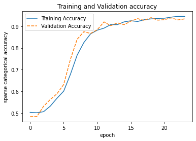
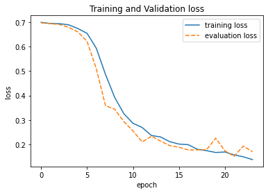
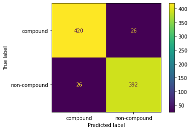
The training curves show stable convergence with minimal overfitting, which is important because this model acts as a routing gate in the pipeline. Misclassifications at this stage propagate downstream, so we prioritize consistency over marginal accuracy gains.
3.4 Western blot detection (EfficientDet-Lite4)
Relevant panels are filtered using a detector.
Without filtering:
- irrelevant images dominate
- retrieval quality drops significantly
After figures are located and routed, the pipeline detects Western blot panels.
The practical benefit is focus:
- downstream embedding extraction and retrieval runs on the blot candidates instead of “everything”.
The repository also documents an explicit consideration of grayscale vs. color for Western blot detection — a reminder that even “small” preprocessing choices can have measurable impact when you deploy.
The detector is reported at Average Precision = 0.797 for the Western blot panels (object detection task). The MVP positions EfficientDet as the primary detection backbone.
3.5 Embedding extraction (BiT / ResNet50‑v2)
Once you have candidate blot regions, you convert them into embeddings that can be searched.
The MVP uses BiT / ResNet50‑v2 embeddings for similarity search. The feature extractor is reported at 94% accuracy (as documented in the performance table below).
ResNet-based models extract feature vectors representing visual content. These embeddings allow similarity comparison instead of pixel matching.
This is where a lot of production skills show up:
- deterministic preprocessing (so embeddings are stable),
- model versioning (so the index doesn’t silently mix incompatible vectors),
- and clean I/O contracts (crop in → embedding out).
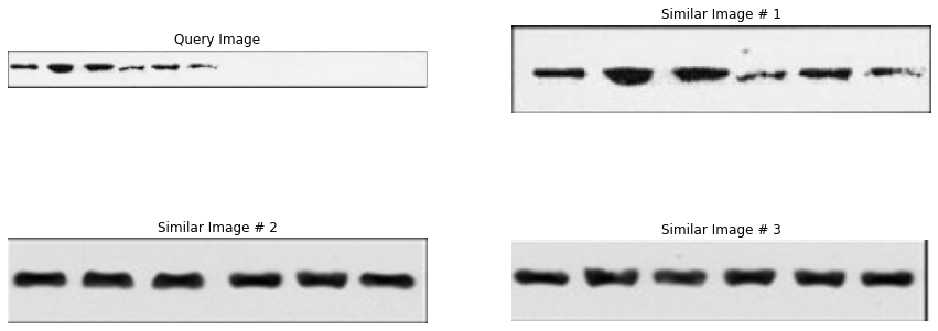
3.6 ScaNN retrieval + reporting
Finally, embeddings are used for near-duplicate search via ScaNN.
ScaNN is an approximate nearest neighbor algorithm. It enables fast similarity search by trading a small amount of accuracy for speed.
At this point, the objective shifts from “is this a duplicate?” to:
“show me the top‑k most similar candidates, with enough context for a human to decide.”
The MVP highlights sub‑millisecond similarity search across large databases, which is exactly what makes the interactive review loop feasible.
Fast retrieval:
- enables interactive workflows
- allows human review
Results are presented as:
- matched panels
- similarity scores
- visual comparisons
4. Cloud Run microservices: why the system is split
The MVP is deployed as separate Cloud Run services rather than a monolith.
Each service:
- has a single responsibility
- can scale independently
The rationale is straightforward:
- independent scaling of compute-heavy components,
- simpler updates and debugging (swap one service without rebuilding everything),
- cost optimization (Cloud Run can scale to zero when idle).
Engineering decision: use Cloud Run
Why:
- automatic scaling
- scale-to-zero (cost efficient)
- simple deployment
4.1 Deployment layout

Even in diagram form, you can see the design intent:
- the Flask web app is the entry point,
- parsing/object orchestration/storage are separate concerns,
- model inference is “outsourced” to TensorFlow Serving endpoints,
- and retrieval is its own service.
4.2 TensorFlow Serving in the loop
The model endpoints are served via TensorFlow Serving.
Separating services:
- improves scalability
- simplifies updates
- isolates failures
Without this:
- one issue can break the entire system
That’s a production-oriented decision:
- inference is isolated from web/business logic,
- models can be updated/versioned without rewriting the app layer,
- and you can scale model-serving instances independently of everything else.
For a multi-stage pipeline, this separation is especially useful: you can tune or replace one model (e.g., figure detection) without touching retrieval.
4.3 Request flow (sequence diagram)
Each stage adds delay.
Too slow:
- breaks user experience
- makes system unusable

5. Performance and validation
The performance's table is deliberately lightweight — but it aligns with the MVP goal (fast reviewer-ready evidence):
| Model | Task | Architecture | Metric | Value |
|---|---|---|---|---|
| Western Blot Detector | Object Detection | EfficientDet‑Lite4 | Average Precision | 80% |
| Feature Extractor | Embedding Generation | ResNet50‑v2 | Accuracy | 94% |
| Compound Classifier | Binary Classification | ConvNeXtTiny | Accuracy | >90% |
In addition, the deployed pipeline can:
- extract figures from PDFs with high accuracy,
- detect Western blot panels,
- generate semantic embeddings,
- perform sub‑millisecond similarity search with ScaNN,
- and scale automatically via Cloud Run.
Key challenges
- latency: each stage adds delay, so we optimized for speed (e.g., efficient models, ScaNN for retrieval).
- consistency: stable inputs/outputs are crucial for reliability, so inconsistent inputs lead to unstable embeddings and break retrieval
- versioning: models change over time. Keep models isolated, versioned: easier updates, avoids breaking the pipeline
What worked
- multi-stage pipeline → reduces complexity
- embeddings + ANN → scalable retrieval
- microservices → flexible deployment
What was harder than expected
- PDF variability → many edge cases
- detection errors → propagate downstream
- balancing speed vs accuracy → constant trade-off
Key insight
Most problems were not model-related — they were system-related.
6. Failure modes and how to debug them
A staged system is easier to debug because each stage has a concrete artifact.
Here are the most common failure categories and where you look first:
-
PDF rendering issues
Symptoms: blank pages, wrong resolution, missing figures.
Debug: render output images and check page dimensions before detection. -
Figure detector misses / false positives
Symptoms: downstream stages see nothing (or too much).
Debug: overlay figure boxes on rendered pages; inspect confidence thresholds. -
Compound routing mistakes
Symptoms: the pipeline treats a compound figure as single-panel (or vice versa).
Debug: inspect classifier outputs on a small curated set of figures. -
Western blot detector over/under-selects
Symptoms: retrieval is noisy (too many non-blots) or empty (missed blots).
Debug: compare color vs grayscale preprocessing choices; inspect detector overlays. -
Embedding drift / index mismatch
Symptoms: retrieval neighbors look random after a deployment update.
Debug: confirm embedding model versioning and that the index was built with the same representation. -
Retrieval returns “visually similar but not duplicates”
Symptoms: top‑k are plausible but not true duplicates.
Debug: review top‑k galleries; tighten thresholds; consider stronger filtering before indexing.
This is the production story in one sentence: make every stage observable with artifacts.
7. Wrap-up and future directions
The key MVP move was not “pick a better model”. It was turn a research pipeline into a deployable system:
- staged CV reduces wasted compute and improves debuggability,
- embeddings + ScaNN make similarity search fast enough for interactive use,
- Cloud Run microservices isolate concerns and scale independently,
- TensorFlow Serving keeps model inference cleanly separated from application logic,
- and the output is shaped for human review — because integrity decisions need context.
The MVP also outlines concrete future work:
- INT8 quantization for faster deployment,
- active learning to bootstrap training data from discoveries,
- multitask detection (figure + blot in one pass),
- transformer detectors (DETR-family),
- enhanced text analysis via deeper LLM integration for caption verification.
Appendix A: Diagram
Series overview (three repos → production MVP)
