From Scientific PDFs to Searchable Evidence for Image-Integrity Checks

January 3, 2024 — Computer Vision Retrieval Data Engineering

This post’s focus: the end-to-end pipeline for turning scientific PDFs into structured, searchable visual evidence. It’s a deep dive into the engineering and model choices that make this possible.

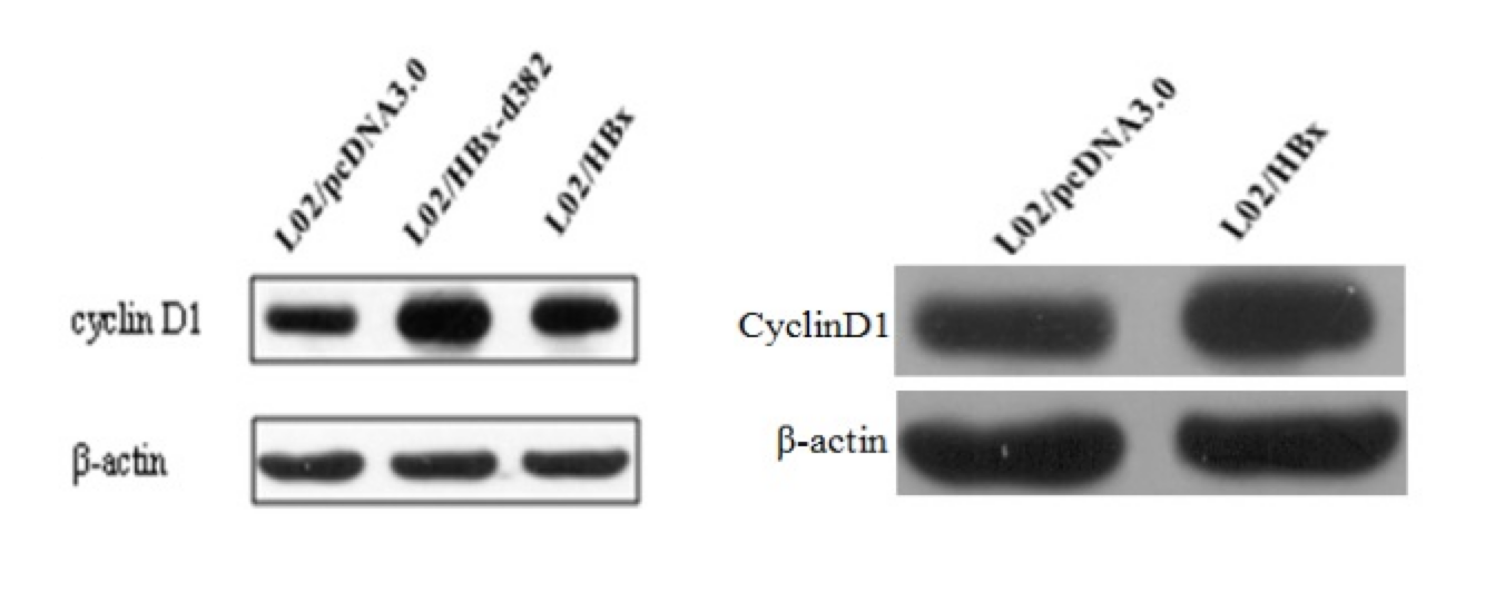
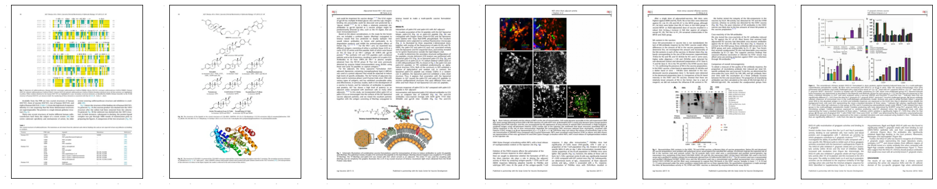
Scientific papers are full of images — figures, charts, microscopy, Western blots. These images often carry the actual evidence behind the claims. But there’s a problem: once published, these images become hard to search, compare, or verify at scale.

If two papers reuse the same image (intentionally or not), detecting that is surprisingly difficult. PDFs are not designed for analysis. Figures are embedded, compressed, and often contain multiple panels. Traditional tools simply don’t work well here.

This post walks through how we turned that messy reality into something searchable: a pipeline that converts PDFs into structured, comparable visual evidence.

Table of contents

1. The problem we’re solving
2. Why scientific image integrity is hard at scale
3. System at a glance
4. Step-by-step: how a PDF becomes searchable evidence
5. Model choices and engineering trade-offs
6. Deployment notes: microservices MVP on Cloud Run
7. What comes next
8. Appendix A: repository map

1. The problem we’re solving

Scientific figure reuse and manipulation are real issues in the literature—especially for image-heavy experimental evidence like Western blots. The practical goal here is not “fully automated misconduct detection”. It’s much closer to:

Given a paper (or a set of papers), surface the most suspicious near-duplicate image matches—fast enough to scale—and package them as evidence for human review.

That “reviewer-first” lens shapes the entire design:

• we need to extract the right visual artifacts from PDFs (and keep their context),
• isolate relevant panels hidden inside compound figures,
• build representations robust to common transformations,
• and search efficiently across a growing corpus.

2. Why scientific image integrity is hard at scale

The “obvious” approach—download images and compare them—breaks quickly in the real world.

PDFs are not clean image datasets

Papers contain:

• compound figures with multiple sub-panels,
• inconsistent caption formatting,
• low-quality extracted images (or missing standalone images),
• and layouts that vary wildly across venues.

So in this project, PDF → figures → panels is a first-class engineering problem, not a preprocessing afterthought. That means building reliable parsing, metadata handling, and reproducible pipelines—skills that look a lot like data engineering, just applied to scientific documents.

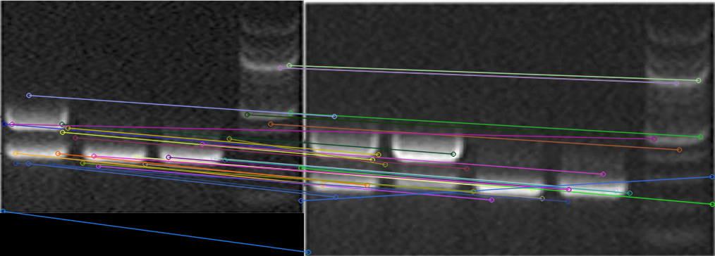
Pixel similarity fails on common transformations

Even simple edits (crop, rotation, rescaling, annotation overlays) can defeat naïve comparisons like MSE. Early prototypes explored:

• classical feature matching (e.g., SIFT) as a sanity-check baseline,
• deep metric learning (a Siamese network with contrastive loss),
• and eventually embedding-based approximate nearest-neighbor retrieval for scale.

Pixel similarity fails under common edits (crop/rotation/annotation), while learned similarity remains stable.

3. System at a glance

At a high level, the end-to-end pipeline looks like this:

1. Ingest PDFs (from open-access sources or upload)
2. Parse pages and extract figures/captions
3. Detect/segment candidate objects inside figures
4. Embed each candidate into a vector space
5. Index & search an ANN structure for near-duplicates
6. Report matches with enough context to review

4. Step-by-step: how a PDF becomes searchable evidence

This section is intentionally procedural: it’s the “how it was done” core.

4.1 Paper discovery and acquisition

For dataset construction, the pipeline queries the Semantic Scholar Academic Graph API to discover open-access papers with downloadable PDFs. The interesting work here is less about “calling an API” and more about building a resilient ingestion job:

• Pagination and filtering (year range, field of study, etc.)
• DOI de-duplication so you don’t re-download the same content
• Checkpointing (saving progress every N papers) so long runs can resume after interruptions
• Rate limiting and practical fault handling

CLI usage (from the repo)

# Query and download papers
python sciImg2Ds.py query "western blot" -y 2020-2023 -f Biology

4.2 PDF parsing and image/caption extraction

After download, PDFs are parsed to extract embedded images and associate them with figure captions. The pipeline does this by converting PDFs into an intermediate structure and then applying targeted heuristics.

Approach

• Convert PDFs to XML using pdftohtml
• Parse the XML to recover image coordinates, dimensions, and page numbers
• Detect captions with heuristics:
  • lines starting with “Fig” / “fig” as caption starts
  • configurable line-height gaps (MAX_LINE_HEIGHT) to find caption boundaries
• Attach caption text + document metadata to each extracted figure

This is a great example of “glue work” skills: PDF tooling, XML parsing, and careful text heuristics to keep figures and captions correctly linked.

CLI usage

# Extract images from downloaded PDFs
python sciImg2Ds.py extract-img pdf/*.pdf

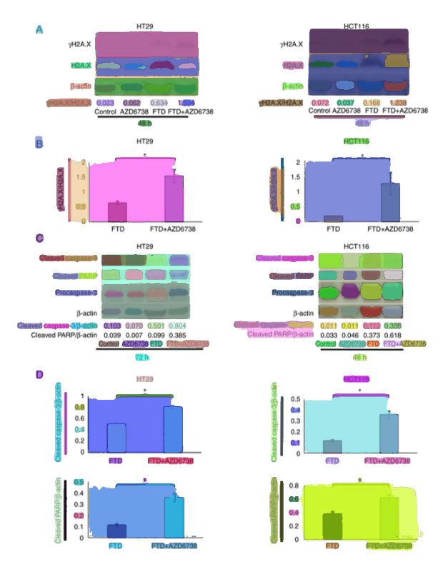
4.3 Object isolation: segmentation and “candidate blot” extraction

Scientific figures are rarely single images. They often contain multiple panels (A, B, C, …), each showing different experiments.

Once you have figures, the next challenge is isolating the objects of interest inside them—especially when a figure contains multiple panels.

For this stage, the pipeline uses Segment Anything (SAM) as a zero-shot segmenter (via Hugging Face Transformers). SAM is a foundation model that can segment objects in images without task-specific training.

Key implementation choices were explicit and reproducible:

• model: facebook/sam-vit-huge
• automatic mask generation via grid-based point prompts (32×32 per side)
• quality filtering:
  • pred_iou_thresh=0.86
  • stability_score_thresh=0.92
• multi-scale mask refinement with crop_n_layers=1
• mask → bounding boxes (so downstream steps can crop candidates cleanly)

The result is a set of candidate crops:

• some are useful (actual panels)
• some are noise

That’s okay. The goal at this stage is high recall, not perfection.

Operationally, this stage also forced practical ML engineering skills: runtime device detection with safe CPU fallback, and memory-aware processing because SAM is compute-heavy.

CLI usage example

# Detect objects in extracted images
python sciImg2Ds.py detect-obj json/*.json

4.4 Representation: embeddings instead of pixels

Once we have image crops, we need a way to compare them.

Direct pixel comparison doesn’t work well:

• small changes break similarity
• resizing or compression alters values

Instead, we use embeddings. Embeddings are numerical representations of images that capture semantic similarity.

Why this matters:

• similar images → similar vectors
• different images → distant vectors

This transforms the problem from “compare images” to “compare vectors”.

After segmentation, each cropped candidate is converted into a vector representation using DINOv2 embeddings. This is the pivot from “compare pixels” to “compare representations”—a core skill shift from classical CV into retrieval engineering.

Implementation details

• model: dinov2_vits14 (ViT‑Small, 14×14 patch) via PyTorch Hub
• preprocessing:
  • square padding (white fill) to preserve aspect ratio
  • resize to 224×224
  • ImageNet normalization
• output: 384‑dimensional embedding per candidate
• storage: embeddings saved alongside metadata in JSON/HDF5 (to support large-scale reads and indexing)

At scale, storage matters. The pipeline explicitly uses HDF5 for efficient columnar storage and partial reads (load only what you need), which becomes important once you’re holding many vectors plus metadata.

CLI usage example

# Extract features from detected objects
python sciImg2Ds.py extract-features json/objectDetected/*.json

Interlude (important): filtering before indexing
Not every segmented panel is a Western blot. To avoid indexing everything, the pipeline evaluates lightweight downstream models on the embedding vectors (e.g., KNN regressor, Histogram‑Gradient Boosting regressor, and a ScaNN-based neighbor approach), with feature scaling (MinMaxScaler) and evaluation via ROC curves / confusion matrices. This is a practical pattern: use expensive foundation models once (to embed), then use cheap models for domain-specific filtering.

4.5 Retrieval: ScaNN similarity search

Once everything is represented as vectors, we can search for similar images.

But there’s another challenge: scale.

If you have thousands (or millions) of image crops, comparing each query against all others becomes too slow.

This is where ScaNN comes in.

ScaNN is an approximate nearest neighbor (ANN) search library. Instead of checking every vector, it:

• partitions the space
• searches only relevant regions
• returns the closest matches efficiently

The trade-off:

• slightly less accuracy
• massively faster queries

For this use case, that trade-off is worth it. We don’t need perfect matches — we need good candidates for human review.

With embeddings in hand, the pipeline builds an approximate nearest-neighbor index using ScaNN. Here, the skills are about tuning retrieval systems: choosing a distance metric, indexing strategy, and recall/speed trade-offs.

Index configuration (as used in the pipeline)

• distance metric: dot product (assumes normalized embeddings)
• tree partitioning: 200 leaves, searching 10 leaves per query
• asymmetric hashing with anisotropic quantization threshold: 0.2
• reordering: 100 candidates for improved accuracy

The key trade-off is explicit: searching only 10 of 200 leaves means ~5% of the index is searched per query, sacrificing some recall for significantly faster queries (the repo notes ~20× faster in this configuration).

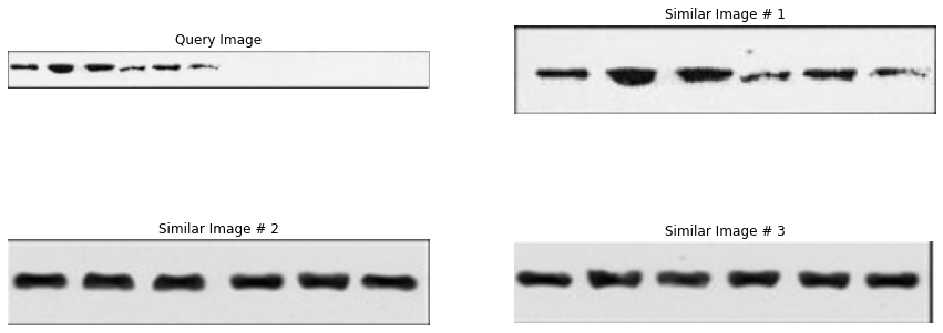
4.6 Reporting: turning matches into reviewable output

Retrieval is only useful if the output is reviewable. In practice, the “reporting” step is where software engineering and product thinking show up:

• include thumbnails / crops and (when useful) bounding boxes
• attach context: paper/page/figure identifiers and caption text
• keep the similarity ranking and a stable link to the underlying source artifacts

That combination lets a reviewer answer quickly: “Is this a true near-duplicate, and is it suspicious?”

5. Model choices and engineering trade-offs

This project is best understood as a sequence of decisions where scale, debuggability, and deployability mattered as much as raw model performance.

• Segmentation vs noise

  More segments = better coverage, but more junk

• Embedding choice

  Better embeddings improve everything downstream

• Search trade-offs

  Faster search can reduce recall

One key insight:

This problem is less about building a perfect model and more about designing a system where each stage supports the next.

Why the solution became multi-stage

Scientific figures are heterogeneous. The project “gates” compute:

1. parse PDFs and keep figure/caption context
2. isolate candidate regions (segmentation or detection)
3. embed candidates once
4. filter to likely Western blots or something else relevant
5. index + search only what matters

That staged design is easier to debug, easier to profile, and makes it practical to replace components when you learn something new (e.g., swap a detector without rebuilding the entire pipeline).

Dataset pipeline vs. production-minded MVP

A useful mental model is that there are two aligned—but not identical—pipelines:

• Dataset pipeline (research/curation)
  Uses pdftohtml parsing, SAM segmentation, DINOv2 embeddings, filtering over embeddings, and ScaNN retrieval. The focus here is building a large, searchable corpus with strong metadata and repeatable extraction.

• Production MVP (service focus)
  Moves toward task-specific models and deployment constraints:

  • EfficientDet‑Lite4 as the chosen Western blot detector (80% accuracy)
  • ConvNeXt (XLarge → Tiny distillation) for compound vs non-compound classification (>90% accuracy)
  • ResNet50‑v2 embeddings used in the similarity pipeline (94% accuracy)
  • ScaNN for fast approximate retrieval (sub‑millisecond retrieval at scale)
  • deployment on Google Cloud Run, with model endpoints via TensorFlow Serving and a Flask web app

The important point isn’t that one is “better”—it’s that different stages optimize for different constraints (data quality and coverage vs. latency/cost/operability).

6. Deployment notes: microservices MVP on Cloud Run

The “production-minded” repository documents a microservices MVP deployed on Google Cloud Run, with models exposed via TensorFlow Serving and an application layer built around a Flask web app. This is where ML meets platform engineering:

• packaging components in containers (Docker)
• separating services so compute-heavy parts scale independently
• leaning on Cloud Run’s autoscaling (including scale-to-zero for cost control)
• treating model serving as an API surface (TensorFlow Serving)

7. What comes next

At this point, we can:

• extract figures from PDFs
• break them into panels
• represent them as vectors
• search for similar images

But there’s still a problem: not all images are relevant.

In the next post, we’ll focus on:

• building a dataset that actually matters
• filtering for specific image types (like Western blots)
• and making retrieval results meaningful

We will dive into the "hard middle" that determines whether the system is usable in practice:

• dataset construction choices (what to label, what to ignore, and why)
• failure modes in parsing and segmentation (and how to debug them)
• retrieval evaluation and thresholding (turning top‑k neighbors into "actionable" candidates)

Appendix A: repository map

This project becomes much clearer when viewed as three phases that matured into separate repos:

1. Research & prototyping

   • similarity baselines (e.g., MSE vs SIFT vs Siamese metric learning)
   • early PDF figure extraction experiments (DETR)

2. Dataset pipeline

   • paper discovery (Semantic Scholar API)
   • PDF → figures/captions (pdftohtml)
   • segmentation (SAM)
   • embeddings (DINOv2)
   • filtering and indexing (ScaNN)
   • FastAPI server + CLI tooling

3. End-to-end + production-minded MVP

   • Western blot detection (EfficientDet‑Lite4)
   • compound figure classification (ConvNeXt distillation)
   • embedding extraction + near-duplicate search (ResNet50‑v2 + ScaNN)
   • Cloud Run microservices + TensorFlow Serving