Building a Western-Blot Dataset and Making Retrieval Actually Work

January 4, 2024 — Computer Vision Dataset Engineering Vector Search

This post’s focus: the “hard middle” — turning messy scientific PDFs into a clean, searchable corpus of Western-blot panels, with practical trade-offs around segmentation, embeddings, labeling, and approximate nearest-neighbor search.

Table of contents

1. Recap
2. The core idea: treat dataset construction as the product
3. Stage 1–2: paper discovery, download, and PDF → figure extraction
4. Stage 3: zero-shot segmentation with SAM
5. Stage 4: embeddings with DINOv2
6. Stage 5: filtering to Western blots
7. Stage 6: ScaNN indexing and retrieval tuning
8. Operational glue: CLI, FastAPI, and long-running jobs
9. What comes next
10. Acknowledgments

1. Recap

In Part 1, we walked the pipeline end-to-end: PDF → figures/captions → candidate panels → embeddings → ScaNN search → report. The key takeaway was that “image integrity” becomes scalable only when you treat both ends seriously:

• upstream: document handling (PDFs are not datasets)
• downstream: retrieval engineering (search is not just a loop over images)

In this post, we focus on the steps that make or break the system’s usefulness:

• extracting figure/caption structure reliably,
• isolating meaningful visual units (panels) with Segment Anything (SAM),
• representing those units with DINOv2 embeddings,
• narrowing the corpus to Western blots with a lightweight labeling loop,
• then tuning ScaNN so nearest-neighbor search is fast and still returns reviewable candidates.

If Part 1 was the map, this post is the “how we actually built the road”.

2. The core idea: treat dataset construction as the product

Most computer vision projects don't fail because of models.

They fail because:

• the data is inconsistent
• the structure is unclear
• and the “dataset” is not actually usable

This project starts with raw scientific PDFs — not clean images — and turns them into a structured, searchable corpus of Western blot panels.

A lot of ML projects treat “dataset” as a prerequisite and “model” as the product. This project flips that: the dataset pipeline is the product. It’s where most of the hard engineering lives:

• API integration + long-running batch execution (downloading papers at scale)
• robust parsing + heuristics (recovering structure from PDFs)
• CV preprocessing and object isolation (turning compound figures into comparable units)
• labeling strategy under scarcity (class imbalance)
• retrieval tuning (fast search without silently ruining recall)

That mindset shows up directly in the repository shape:

• dedicated modules (downloader.py, parser.py, object_detector.py, feature_extractor.py, io.py)
• a CLI (sciImg2Ds.py) built with Click + Rich (progress + logging)
• a FastAPI server (server.py) for interactive runs
• scripts for pseudo-labeling and fast manual labeling (autolabel.py, fastLabel.py)

3. Stage 1–2: paper discovery, download, and PDF → figure extraction

At first glance, this looks like a standard CV problem:

• detect objects
• compare images
• find duplicates

In reality, the challenge is upstream:

PDFs are not datasets.

They are:

• inconsistent layouts
• mixed text and images
• compound figures
• and missing structure

So before any model works, you need to:

• recover structure
• define meaningful units (panels)
• and create a dataset that supports retrieval

Why this mattered

Without a clean dataset:

• segmentation becomes noisy
• embeddings become meaningless
• retrieval results become unusable

3.1 Semantic Scholar bulk search

The pipeline starts at the corpus layer: discover and download open-access PDFs via the Semantic Scholar Academic Graph API, using bulk search (/paper/search/bulk) with token-based pagination.

We've had a pure “production data work” in this stage:

• query design (repeatable slices by year/field/venue)
• pagination and resumability (token handling + checkpointing)
• DOI-based de-duplication (don’t waste compute reprocessing the same paper)
• respectful rate limiting (so the run doesn’t self-DOS)

3.2 Caption alignment heuristics

After download, the parser’s job is to associate extracted images with the right caption text. That sounds straightforward until you hit real PDFs:

• multi-line captions with inconsistent spacing,
• “Fig.” / “Figure” variations,
• multiple subfigures sharing one caption (compound figures),
• and page layouts that aren’t consistent even within one journal.

The approach is intentionally heuristic:

• detect caption starts (e.g., lines beginning with “Fig” / “fig”),
• use line-height gaps (configurable MAX_LINE_HEIGHT) to decide caption boundaries,
• then attach captions to candidate images by proximity and layout cues.

This is one of those places where “simple” logic + good thresholds beats a fragile overfit system, especially when you need predictable failure modes and quick debugging.

Why this mattered

Captions provide context:

• what the figure represents
• how panels relate to each other

Without this:

• filtering becomes harder
• interpretation becomes ambiguous

3.3 Why pdftohtml (and what it buys you)

Tool choice matters here. The pipeline uses pdftohtml (Poppler) to convert PDFs into XML and extract embedded images as separate files.

This decision is less about “the best parser in theory” and more about maintainability:

• file-based outputs are easy to inspect when extraction fails,
• XML makes layout-driven heuristics easier than raw byte-stream hacking,
• and the extracted images become stable artifacts for downstream steps.

4. Stage 3: zero-shot segmentation with SAM

Once you have extracted figures, you need a reliable “comparison unit”.

Compare whole figures and you’ll miss duplicates inside compound figures. Compare arbitrary crops and you’ll drown in noise. The compromise is to generate candidate regions automatically, then filter downstream.

SAM is a foundation model that can segment objects in images without task-specific training. SAM is used as a panel-proposal engine: generate candidate masks without requiring segmentation labels.

4.1 Automatic mask generation parameters

The implementation uses Hugging Face Transformers with facebook/sam-vit-huge and automatic mask generation with grid-based prompts:

• points_per_side = 32 (32×32 grid)
• quality filters:
  • pred_iou_thresh = 0.86
  • stability_score_thresh = 0.92
• multi-scale: crop_n_layers = 1

The “skill” here isn’t just calling SAM — it’s tuning the pipeline so it produces useful candidates:

• lower thresholds increase recall but inject noise,
• higher thresholds reduce noise but risk missing sub-panels,
• and the right defaults are the ones you can defend when you inspect overlays.

Engineering decision: prefer high-quality masks

We use relatively strict thresholds to reduce noise.

Why this mattered

Too many segments:

• noisy crops
• poor embeddings

Too few segments:

• missed panels

This balance directly impacts retrieval quality.

4.2 Mask → bounding box, plus augmentation

Once panels are extracted, they need to be comparable.

Accepted masks are converted to bounding boxes, then cropped for downstream embedding extraction. The pipeline also applies a small random perturbation (0–10px) to bounding boxes as a simple augmentation.

This step is small but foundational:

• crops become standardized artifacts you can store, re-embed, and index,
• perturbation builds robustness against minor localization errors,
• metadata links keep every crop traceable back to the source paper/page/figure.

4.3 Compute and memory reality (CUDA, sequential processing)

SAM + DINOv2 are heavy. The pipeline detects acceleration (CUDA) and falls back to CPU if needed.

More importantly, it includes practical memory controls:

• processing images sequentially (not batched),
• skipping tiny images (e.g., <64×64),
• deleting intermediate tensors explicitly.

These are the kinds of operational choices that determine whether a pipeline runs for minutes or quietly dies after hours.

5. Stage 4: embeddings with DINOv2

After segmentation, each crop is mapped into a vector representation using DINOv2.

5.1 Preprocessing and storage format

The feature extractor uses PyTorch Hub with dinov2_vits14 and produces 384‑dimensional embeddings.

Preprocessing is explicit and consistent:

• square padding (white fill) to preserve aspect ratio,
• resize to 224×224,
• ImageNet normalization.

Embeddings and metadata are stored as compact artifacts (JSON/HDF5 via h5py), which makes later steps (filtering, indexing, evaluation) much easier to automate and reproduce.

5.2 Why embeddings unlock scale

Moving from pixel comparisons to embeddings enables three things at once:

1. robustness to common transforms (crop/resize/contrast shifts)
2. searchability via vector similarity
3. separation of concerns: segmentation can improve without changing retrieval logic; retrieval can be tuned without reworking extraction

This is the core “CV → retrieval engineering” pivot of the project.

6. Stage 5: filtering to Western blots

If the target is Western-blot reuse, the pipeline should filter early. Otherwise, the index fills with charts, microscopy images, diagrams, and retrieval quality collapses.

Not all extracted panels are relevant.

Western blots are a minority class, so filtering is essential.

6.1 Class imbalance and why “filter first”

Western blots are a minority class, so the pipeline explicitly designs for imbalance:

• build a small labeled seed set,
• train a classifier on embeddings,
• then triage new candidates for labeling and indexing.

This is the common applied-ML truth: you don’t get a balanced dataset by wishing for it — you get it by designing a labeling loop.

Instead of training from scratch:

• reuse embeddings
• train lightweight models (KNN, HGB)

6.2 Human-in-the-loop: fastLabel.py + autolabel.py

Two scripts capture the practical labeling approach:

• fastLabel.py: interactive manual labeling for rapid bootstrapping
• autolabel.py: pseudo-labeling to expand coverage (with verification focused on edge cases)

This is a strong “skills story” in one place:

• build the smallest UI needed to create ground truth,
• automate the boring middle,
• then spend human effort where uncertainty is highest.

Why this mattered

Manual labeling alone does not scale.
Pure automation is unreliable.

The combination:

• speeds up dataset growth
• keeps quality under control

6.3 Model choices: KNN vs HGB (and how we evaluate)

We've tried multiple candidates for the “Western blot vs other” filter:

• KNN Regressor
• Histogram Gradient Boosting Regressor (HGB)
• Random Forest
• nearest-neighbor approaches using ScaNN

Embeddings are scaled via MinMaxScaler, and models are persisted (e.g., knr.joblib) so the filter becomes a reusable pipeline component.

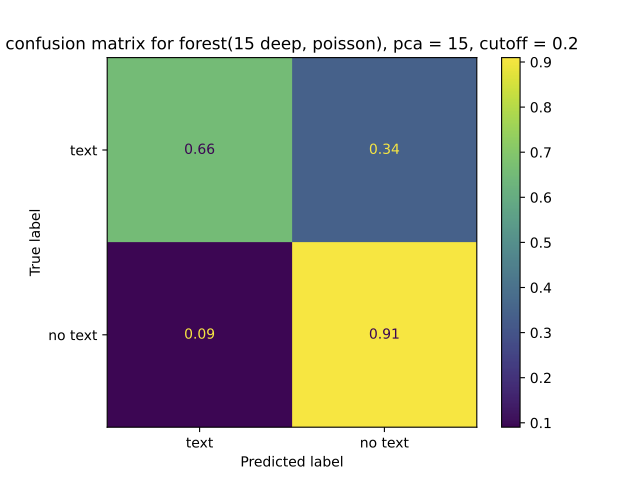
Evaluation focuses on what matters under imbalance:

• ROC curves
• confusion matrices
• prediction histograms

Engineering decision: start with KNN

Why:

• simple and interpretable
• strong baseline with good embeddings
• minimal tuning required

7. Stage 6: ScaNN indexing and retrieval tuning

Once you have a Western-blot-focused embedding set, you can build an approximate nearest-neighbor index to support fast similarity queries.

Exact search is too slow at scale.

ScaNN:

• partitions data
• searches a subset
• re-ranks candidates

7.1 The index configuration used

The documented ScaNN configuration is:

• distance: dot product (assumes normalized embeddings)
• partitioning: 200 leaves, searching 10 leaves per query
• asymmetric hashing with anisotropic quantization threshold = 0.2
• reordering: 100 candidates

This is retrieval engineering in practice: tune the system so it returns useful candidates quickly enough for an interactive review workflow.

7.2 Speed/recall trade-offs in plain terms

With num_leaves=200 and num_leaves_to_search=10, the query inspects only ~5% of partitions. That’s why it’s fast — and why it’s approximate.

The right trade-off depends on the product goal:

• if you want “a few strong suspects quickly” for human review, speed wins,
• if you need maximum recall (e.g., for offline audits), you’ll search more leaves and accept latency.

Why this mattered

Faster queries:

• enable interactive workflows
• allow rapid inspection

Slightly lower recall:

• acceptable for human-in-the-loop review

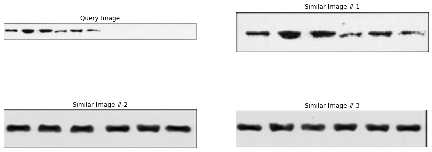
7.3 What “good retrieval” looks like in practice

For integrity review, “good retrieval” is a workflow outcome:

• top‑k neighbors should include plausible duplicates even after small transforms,
• similarity scores should be stable enough to threshold,
• and failures should be inspectable (so you can improve extraction, filtering, or index tuning).

A practical evaluation loop is:

1. pick query panels from known papers
2. inspect top‑k neighbors
3. label outcomes as:
   • near-duplicate
   • visually similar but different (false positive)
   • missed match (false negative)
4. adjust:
   • segmentation thresholds,
   • filtering threshold,
   • ScaNN parameters,
   • or post-processing rules

The key skill here is closing the loop: building a system you can debug with artifacts (overlays, crops, neighbors), not guesses.

7.4 What actually mattered (lessons learned)

Several things had outsized impact:

Dataset quality > model complexity

Better segmentation and filtering improved results more than changing models.

Good defaults > aggressive tuning

Caption alignment and thresholds had a big effect on downstream quality.

Filtering is critical

Without filtering:

• retrieval becomes noisy
• results lose meaning

Retrieval is an engineering problem

It is not just:

• “compute similarity”

It is:

• representation
• indexing
• and trade-offs

8. Operational glue: CLI, FastAPI, and long-running jobs

A pipeline like this succeeds or fails on operational details:

• it has to run for hours/days,
• survive crashes,
• and produce artifacts you can resume from.

This repo includes several signals of “engineering maturity”:

• a CLI built with Click + Rich (progress bars, logging),
• a FastAPI web application with endpoints to run the pipeline interactively,
• Google Cloud integration (GCS bucket sci-images-dataset, Compute Engine Tesla T4, Cloud Logging),
• and operational “quality of life” features such as email notifications (gmail.py).

The CLI runbook examples

# Query and download papers
python sciImg2Ds.py query "western blot" -y 2020-2023 -f Biology

# Extract images from downloaded PDFs
python sciImg2Ds.py extract-img pdf/*.pdf

# Detect objects in extracted images
python sciImg2Ds.py detect-obj json/*.json

# Extract features from detected objects
python sciImg2Ds.py extract-features json/objectDetected/*.json

# Run full pipeline
python sciImg2Ds.py all "western blot" -y 2020-2023

9. What comes next

This dataset pipeline enables the final step:

turning the system into a production-ready service

In the post 3 we move from the dataset pipeline to the production-minded MVP:

• how multi-stage detection/classification changes the failure modes,
• how model serving + microservices shape performance and cost,
• and how the system packages matches into reviewer-friendly evidence.

10. Acknowledgments

Special thanks to Fabian Schierok, who worked with me on the dataset pipeline.