Automated Grain Segmentation for Rock Thin Sections: From U-Net Baselines to Segment Anything

September 12, 2023 — Research Computer Vision Petrology

Petrographic thin‑section analysis depends heavily on grain geometry — size, orientation, and shape often underpin geological interpretations.
Extracting those measurements manually is slow and subjective.

This project explores how computer vision can convert microscope imagery into structured, measurable grain data through automated segmentation and geometric analysis.

Table of Contents

1. Overview
2. Defining a Practical Goal
3. Building a Dataset Pipeline
4. Establishing Baselines
5. Pivoting to Segment Anything (SAM)
6. From Segmentation to Measurement
7. Early Deployment Experiments

Overview

Thin‑section petrography contains a surprising amount of geometry.
Grain size distributions, orientation patterns, and elongation can provide insights into:

• deformation history
• sediment transport processes
• rock fabric development
• proxies sometimes used in porosity or permeability estimation workflows

The difficulty is not the mathematics — it is the image interpretation.

Separating individual grains in dense thin‑section imagery is tedious and error‑prone when performed manually. This project investigates a workflow that automates the first part of that process:

1. Segment mineral grains from microscope images
2. Convert segmentation masks into measurable geometric properties

The result is a pipeline that transforms raw imagery into structured data suitable for downstream geological analysis.

Defining a Practical Goal

Image segmentation is a computer‑vision task that assigns a label to every pixel in an image.

Instead of predicting a single class for the entire image, segmentation produces a mask that identifies regions belonging to objects of interest.

For thin‑section imagery, segmentation allows each mineral grain to become a distinct measurable object.

The project began by defining a practical outcome rather than a specific model target.

A useful system would need to:

• reliably identify grain boundaries
• avoid merging adjacent grains
• produce masks suitable for geometric measurement

That last constraint is important: segmentation accuracy is only meaningful if the resulting masks can support stable downstream measurements.

Building a Dataset Pipeline

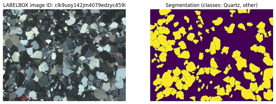
The training data consisted of microscope images paired with segmentation masks.

These masks represent grain boundaries drawn by annotators.

Technology: LabelBox

LabelBox is an annotation platform frequently used in machine‑learning workflows.
It provides tools for drawing masks or polygons directly on images and offers APIs for exporting labeled datasets.

Engineering Decision

Treat annotation storage as the system of record

Instead of exporting labels manually, the dataset pipeline retrieves annotations through the LabelBox API.

The pipeline:

1. fetches annotations
2. converts them into mask images
3. generates reproducible train/validation splits

Early automation in dataset preparation reduces friction later in experimentation.
Reproducible splits make it easier to compare experiments and understand whether changes actually improve results.

Establishing Baselines

Before exploring newer architectures, the project started with U‑Net, a widely used segmentation architecture.

U‑Net is a convolutional neural network designed for segmentation tasks.

Its architecture consists of:

• an encoder that extracts hierarchical visual features
• a decoder that reconstructs spatial detail
• skip connections that preserve fine structure

This design allows the network to combine contextual understanding with precise boundary prediction.

Baseline Experiment 1 — TensorFlow U‑Net

The first training run served primarily to validate the full pipeline.

Configuration:

• TensorFlow implementation
• Sparse categorical cross‑entropy loss
• ~100 training epochs

At this stage the emphasis was less on maximizing performance and more on ensuring that:

• images and labels aligned correctly
• training proceeded without instability
• segmentation outputs were plausible.

Baseline Experiment 2 — PyTorch U‑Net

A stronger configuration followed using PyTorch.

segmentation_models_pytorch is a library providing high‑quality implementations of common segmentation architectures with pretrained encoders.

Configuration:

• EfficientNet‑B0 encoder (ImageNet pretrained)
• Dice + BCE loss combination
• Adam optimizer
• 640×640 input resolution
• extended training schedule

Engineering Decision

Use pretrained encoders

Pretrained encoders reuse visual features learned from large image datasets such as ImageNet.

Thin‑section datasets are relatively small compared with natural‑image datasets.
Transfer learning helps models converge faster and improves boundary detection in many cases.

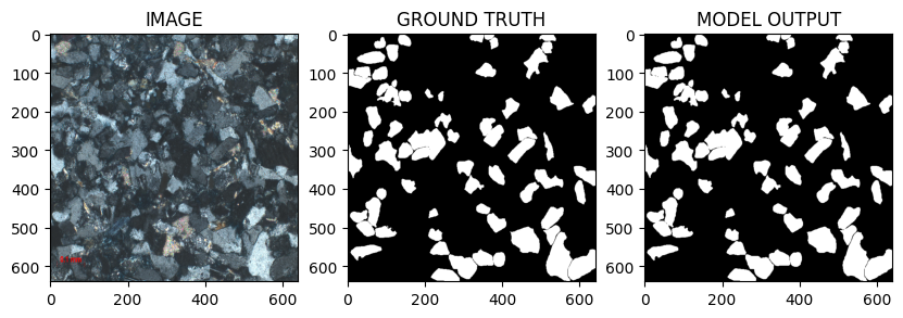
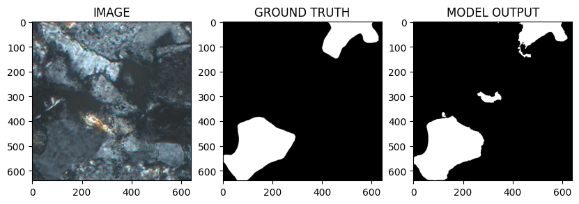
Observed Failure Mode — Merged Grains

Despite stronger training setups, a persistent issue appeared:

adjacent grains frequently merged into single blobs.

Merged grains compromise the measurements derived from segmentation.

If multiple grains appear as one object:

• area becomes incorrect
• orientation becomes meaningless
• size distributions become distorted

Addressing this limitation became the central modeling challenge.

Pivoting to Segment Anything (SAM)

Rather than refining a custom segmentation architecture indefinitely, the project explored Segment Anything (SAM).

Segment Anything is a foundation segmentation model released by Meta.

Key characteristics:

• trained on an extremely large segmentation dataset
• designed to generalize across domains
• capable of producing masks for many object types

The model uses a Vision Transformer (ViT) backbone rather than a traditional CNN.

Engineering Decision

Evaluate a foundation segmentation model

Instead of continuing incremental improvements to U‑Net, SAM provided a different starting point: a model trained to recognize boundaries across diverse visual domains.

Boundary preservation — particularly between touching objects — is critical in grain segmentation.

Foundation models sometimes capture these structures more robustly than smaller task‑specific networks.

SAM Experimentation Workflow

The evaluation followed several stages.

1. Zero‑shot evaluation

Initial tests explored how well SAM handled thin‑section imagery without additional training.

2. Fine‑tuning

The model was then adapted to the dataset using:

• PyTorch
• Hugging Face Transformers
• MONAI loss functions

3. Visual evaluation

Outputs were inspected primarily for:

• boundary consistency
• grain separation quality
• segmentation stability.

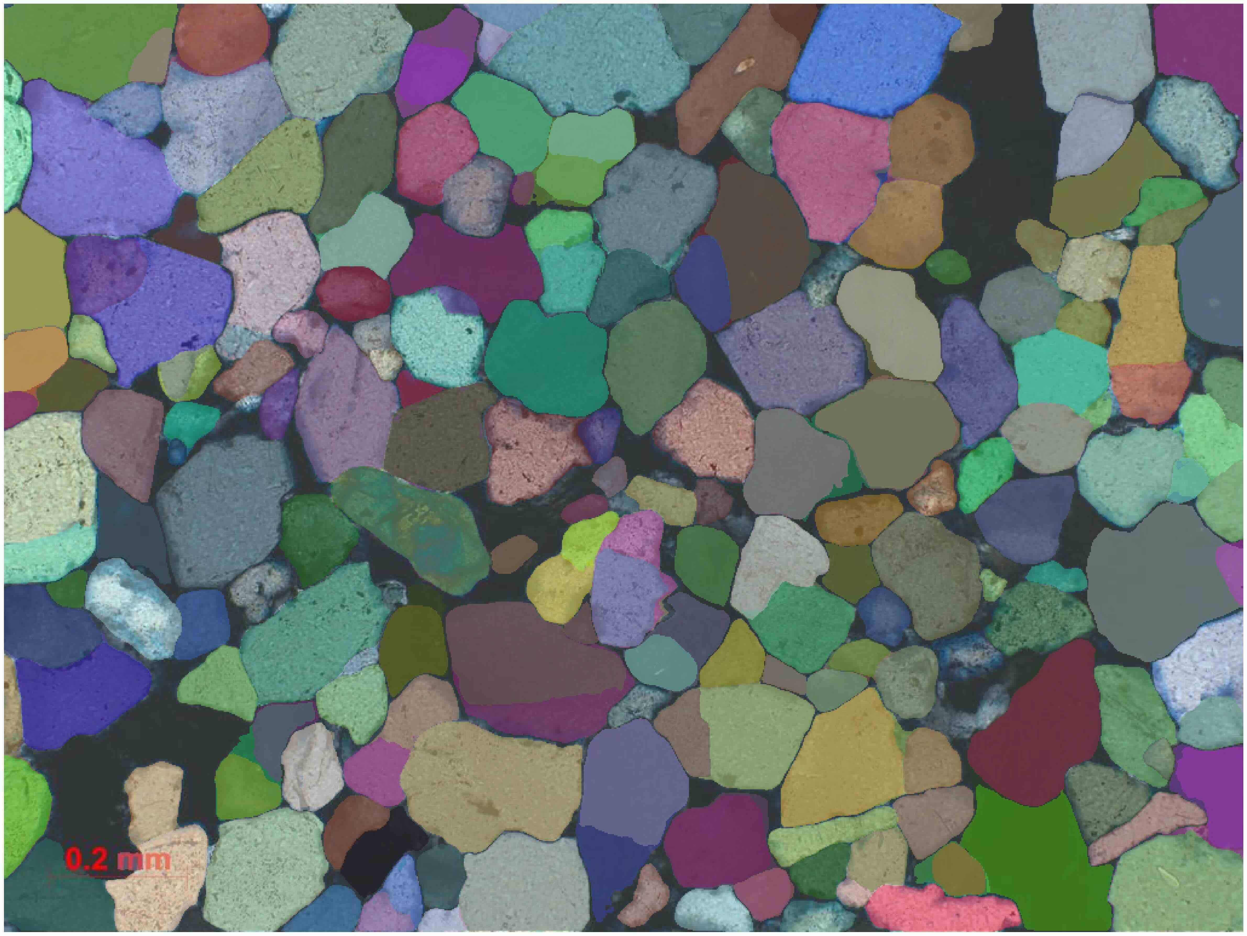
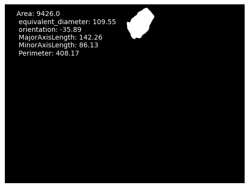
From Segmentation to Measurement

Once grains are segmented, masks become geometric objects.

scikit-image is a Python library for image analysis.
Its regionprops function extracts measurements from labeled mask regions.

Examples of extracted properties:

• area
• centroid
• orientation
• eccentricity
• major and minor axes

These metrics form the bridge between computer vision output and geological interpretation.

In the service implementation, the same idea is expressed as per-object feature extraction (area/perimeter, equivalent diameter, major/minor axes, orientation), computed from each binary mask region.

Early Deployment Experiments

While the primary focus of this phase was experimentation, the workflow was also tested outside a notebook environment.

Initial experiments included:

• packaging inference with TorchServe
• running tests on Google Cloud infrastructure

These early checks helped confirm that the segmentation pipeline could realistically operate as part of a larger system.

What Comes Next

This post described the research and experimentation phase:

• dataset creation
• segmentation baselines
• the pivot toward foundation segmentation models
• converting masks into geological measurements

The next post focuses on the engineering side: turning this workflow into a GPU‑backed API capable of processing images asynchronously in the cloud.

← Read Post 2: Productionizing SAM Segmentation: A GPU-Backed Async API on Google Compute Engine